How to Add in Google Sheets: SUM and MINUS Formulas

Key takeaways

To perform calculations in Google Sheets, you must first enter the function you wish to execute. 

• The formula to add in Google Sheets is =SUM(value1, [value2, ...]).

• The formula to subtract in Google Sheets is =MINUS (value1, value2).

• You can add and subtract numbers, cells, or a range of cells in Google Sheets using these two functions. 

Learn how to work with both of these functions by exploring how to use the SUM and MINUS functions to perform a variety of actions in your Google Sheets. If you're ready to gain in-demand skills in Google Workspace, try the Getting started with Google Workspace Specialization to learn about Google Docs, Sheets, Slides, Calendar, and how to collaborate with others across the workspace. 

SUM and MINUS formulas

The SUM syntax is:

=SUM(value1, [value2, ...])

• value1: The first number, cell, or range to add

• value2: (Optional) the second number, cell, or range to add

The MINUS syntax is:

=MINUS (value1, value2) 

• value1: the number, cell, or range to be subtracted from 

• value2: the number, cell, or range to subtract 

Ready to deepen your knowledge of Google Sheets?

To begin, you'll need your tab open to your Sheet. If you’re not already working with your own data set and want to follow along with the examples below, make a copy of this template to practice.

How to add in Google Sheets

When you want to find the sum total of data in Google Sheets, you can add cells or an entire column together using the SUM function. 

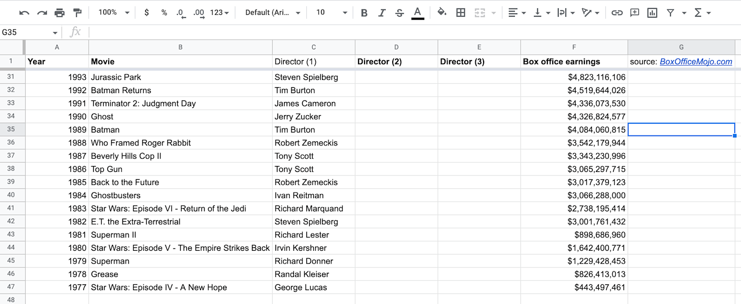
1. Choose an empty cell where you’d like the sum to appear.

As an example, you can use SUM to understand more about the column Box Office Earnings in your practice sheet. You could choose a cell at the end of the Box Office Earnings column, or you could choose a cell next to the data you want to add. 

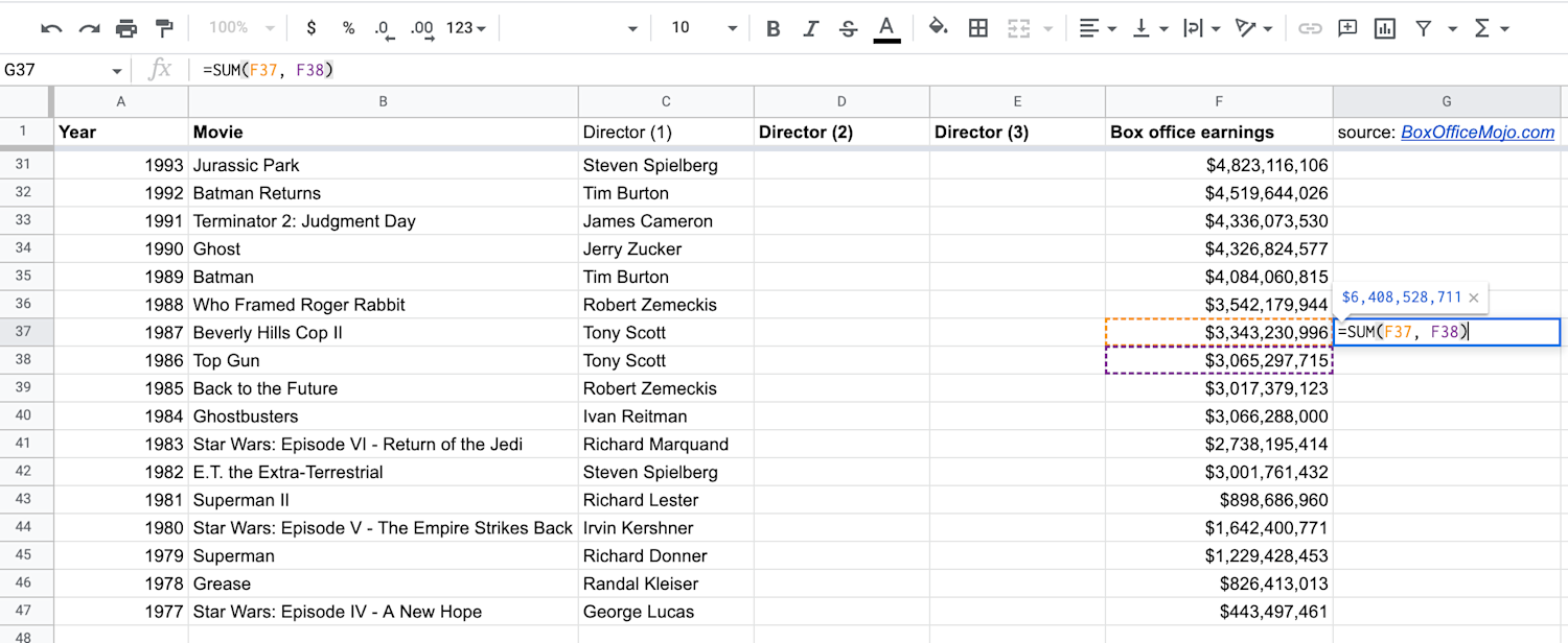
2. Use the SUM function to add two cells.

When you begin to type “=SUM” into an empty cell, Google Sheets will automatically display the SUM function =SUM(value1,value2). The comma here tells Sheets to add these values together. Values can be specific cells, numbers, or ranges. 

To add two cells, your two values will be the cells you want to total. For example, =SUM(A2, A3) will add cells A2 and A3. Or =SUM(A2, A3, A4) will add cells A2, A3, and A4. 

For practice, you can have Sheets SUM the movies directed by Tony Scott in the 1980s, which are rows F37 and F38. In that case, your function should read =SUM(F37, F38). With that function, you get the total earnings for his 1980s films, Top Gun and Beverly Hills Cop II.

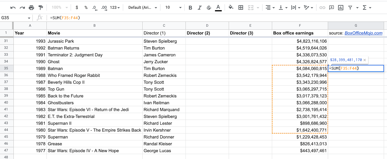
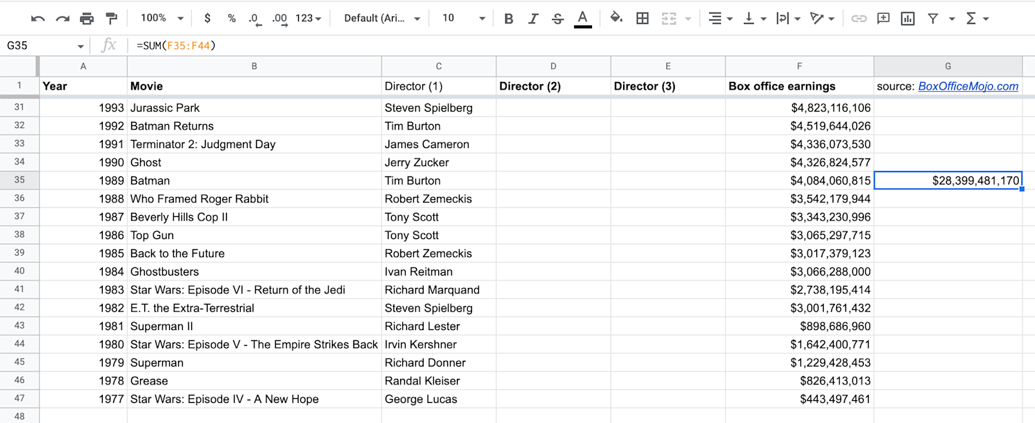
3. How to add up a column in Google Sheets.

In another scenario, you might want to find the total for a range of cells (which also works for an entire column). In that case, you’d only need to define one value in your SUM function, and that value will be a range: =SUM(value1). A range is written as two cells separated by a colon, [first cell]:[last cell].

For practice, you can add together all movies in the 1980s, or F35 to F44. Your formula should be =SUM(F35:F44). 

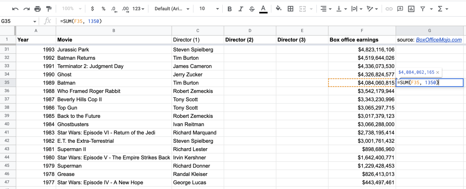
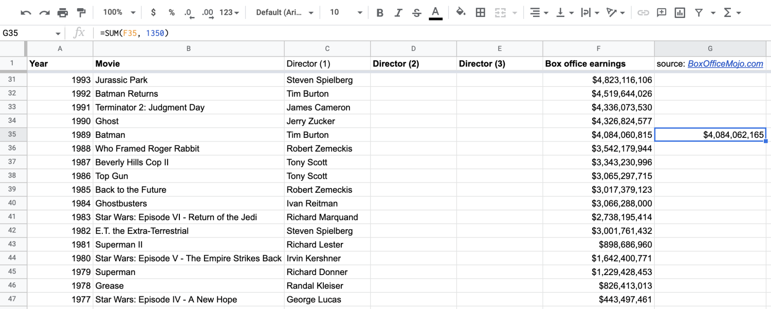
4. Use the SUM function to add a specific number.

If you want to add a specific number to data you’ve accumulated, you can use a number as one of your values.

For example, if you want to find out what an extra $1,350 in ticket sales would add to 1989’s Batman, the function would become =SUM(F35,1350).

How do you sum in Google Sheets?

If you're wondering how to add numbers in Google Sheets quickly, follow these steps:

1. Highlight the cells you plan to add.

2. In the bottom right of your Google Sheet, locate Sum: (your total).

3. Click Sum: (your total), and a submenu will appear where you can view other figures like:

- Average

- Minimum

- Maximum

- Count

- Count numbers

Note: This feature does not apply to some currency types and certain numbers.

How to subtract in Google Sheets

Similar to the SUM function, you can use the MINUS function to figure out the difference between two cells or an entire column.

1. Choose an empty cell where you’d like the difference to appear. 

As with SUM, you can choose whichever empty cell makes sense—something besides a row of numbers or at the end of a column of numbers. 

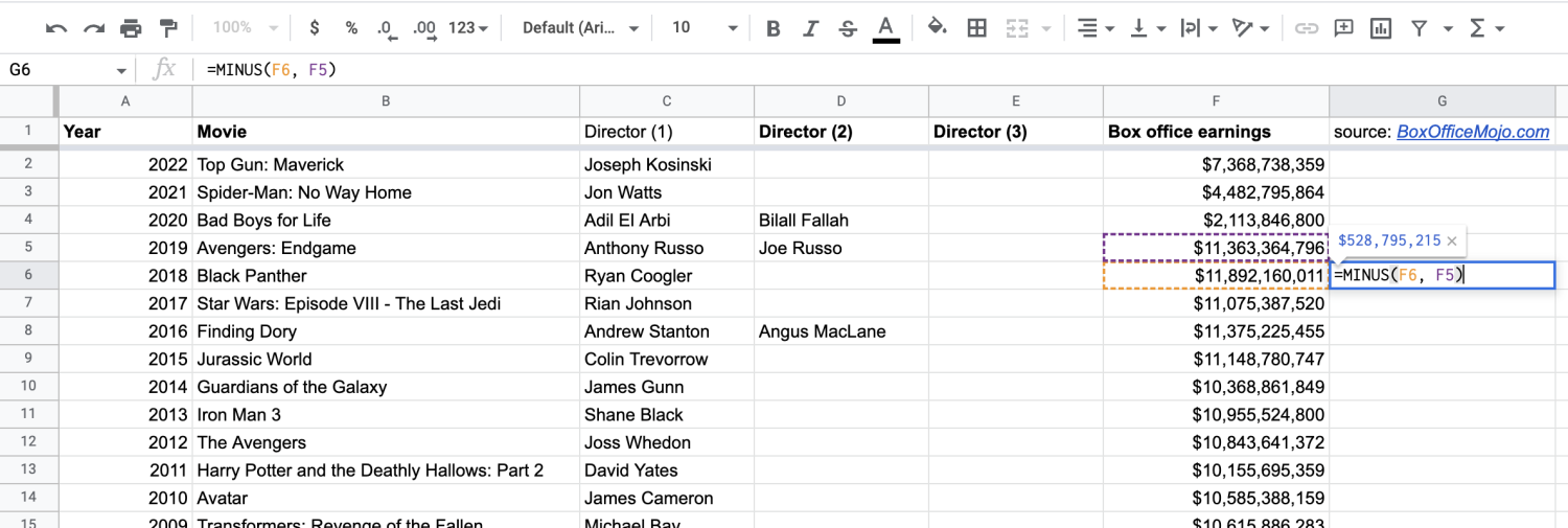
2. Use the MINUS function to subtract cells. 

When you begin to type “=MINUS” into an empty cell, Google Sheets will automatically populate the MINUS function =MINUS(value1,value2). The comma here once again tells Sheets to subtract these values. Note that the MINUS function can only handle two values, and your values can be specific cells, numbers, or a range.

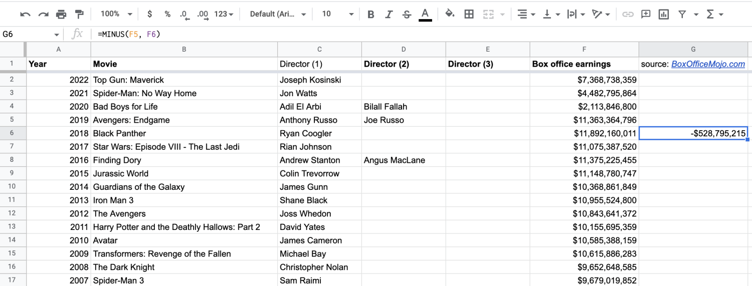
To subtract two cells, your values will be your two cells. For example, maybe you want to find out how much more Blank Panther grossed compared to Avengers: Endgame. Your function then becomes =MINUS(F6, F5) because, according to the Google Sheet, you know Black Panther (F6) made more, and you want to subtract Avengers (F5). 

If you subtracted F5 from F6, you’d get the same number, but it should show a negative quality because Avengers didn’t earn as much. 

3. Subtract multiple cells from the total of one cell.

If you’d like to subtract multiple cells from the total of one cell, you’ll need to use the subtract formula and the SUM function. (The MINUS function won’t help here because it’s designed to look at the difference between no more than two values.) 

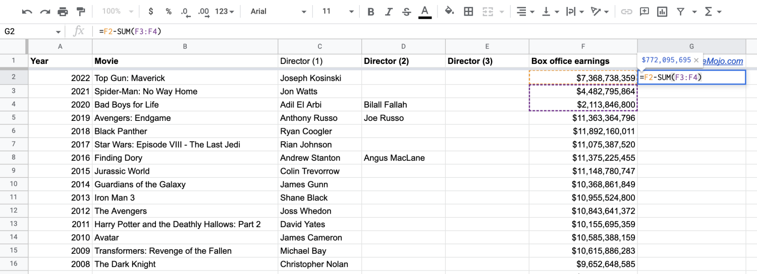
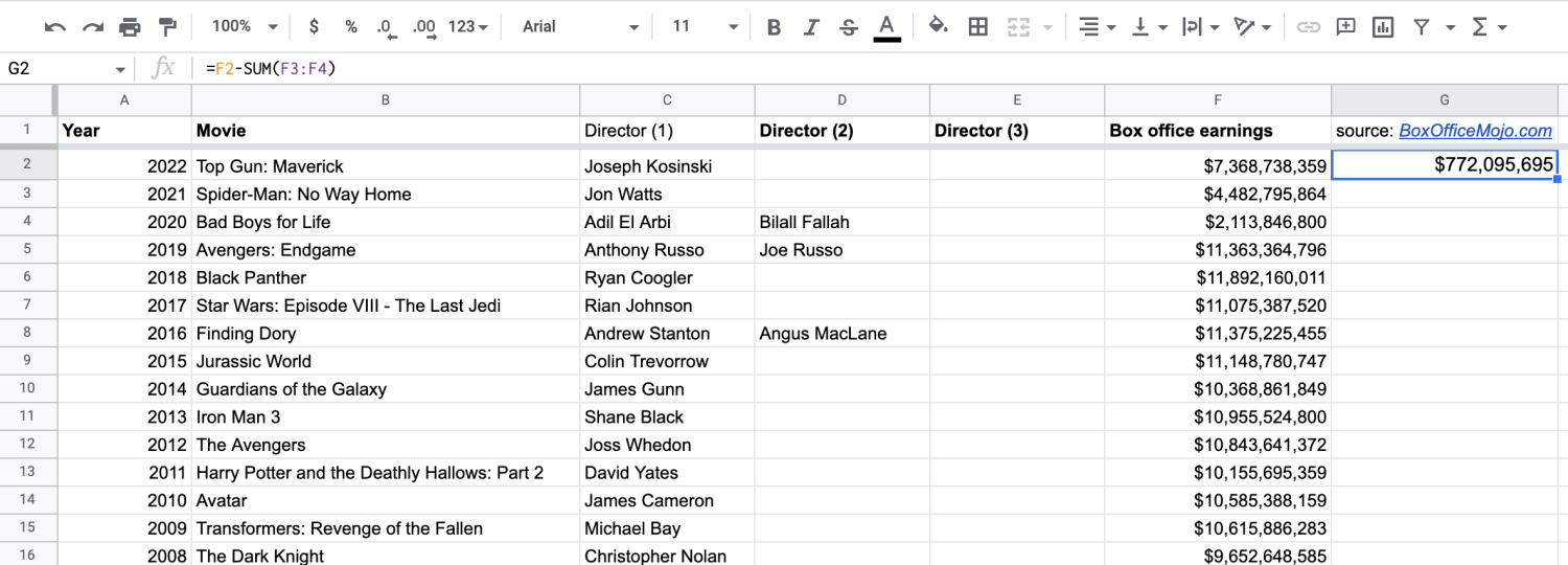
The formula to subtract multiple cells from one cell is =value1-SUM(value2,value3). This tells Sheets to add together your second and third values and subtract the sum from the first. 

For example, you can add together Bad Boys for Life and Spider-Man: No Way Home, and subtract them from Top Gun: Maverick. Your formula then becomes =F2-SUM(F3:F4).

How to copy the SUM and MINUS functions to an entire column

There may be times when you need to apply the SUM or MINUS functions to an entire column, capturing the total or difference of two or more cells for each row. Fortunately, there's a straightforward way to copy the SUM function and apply it to an entire column. Take a look at how to sum columns in Google Sheets.

1. Add the function to your first cell.

Maybe you want to sum columns A and B in Google Sheets to understand the relationship between each row. Start by adding the SUM function to your first cells, A2 and B2. (The steps are the same for the MINUS function.) 

2. Double-click the small blue box.

You’ll notice a small blue box appear in the bottom right corner of your highlighted cell. Double-click it to apply the function to the entire column.

Read more: How to Import XML to Google Sheets

Common SUM and MINUS errors and solutions

The issues below most commonly arise when using SUM or MINUS. If you’re not getting the information you want, use the following tips:

• #N/A error: The MINUS function can only handle two values, so if you try to add more, such as by subtracting a range, you’ll see #N/A because Sheet was expecting two values (or “two arguments,” as it will explain) and it got more than that. 

• If the function doesn’t populate an answer or you get “0” as your total: You might have text somewhere in your cells. For instance, Sheets reads currency symbols as text, so adding cells or columns denoting currency ($25 or £100) may create an error. 

Double-check to make sure you’re adding or subtracting only numerical values. 

• Clearing one function before using another: If you want to apply a function to an entire column that already has an existing function, you’ll have to first clear that data before Sheets will apply the new function. 

Explore our free resources for Google Sheets and data analytics

Subscribe to our Career Chat newsletter on LinkedIn for industry insights, skill-building tips, and networking opportunities. Then, explore our free resources for learning Google Sheets: 

• Learn new techniques: Google Sheets Automation: A Step-by-Step Guide 

• Take a quiz: Data Science Career Quiz: Is It Right for You? Find Your Role 

• Hear from an expert: 7 Questions with a Data Analytics Professor

Accelerate your career growth with a Coursera Plus subscription. When you enroll in either the monthly or annual option, you’ll get access to over 10,000 courses. 

订阅 Coursera Plus，培养就业技能

开始为期 7 天的免费试用

• 
• 
• 
• 

开始为期 7 天的免费试用