How to Highlight Duplicates in Google Sheets

Key takeaways

• When you're dealing with a large data set, you may sometimes want to double-check and make sure no duplicates exist.

• Or you may want to highlight any duplicates to call attention to them.

• There's a straightforward formula in Google Sheets that will highlight duplicates if any exist.

Learn how to find duplicates in Google Sheets with step-by-step instructions. Afterward, learn how to filter, summarize, and protect data in the Google Sheets course.

How to highlight duplicates in Google Sheets

Highlighting duplicates in Google Sheets requires conditional formatting using the custom formula =COUNTIF (A:A, A1)>1. Follow these steps to learn how to use it.

Practice with Google Sheets: Highlight duplicates

To begin, you'll need your tab open to your spreadsheet. If you’re not already working with your own data set and want to follow along with our examples, make a copy of this template to practice. 

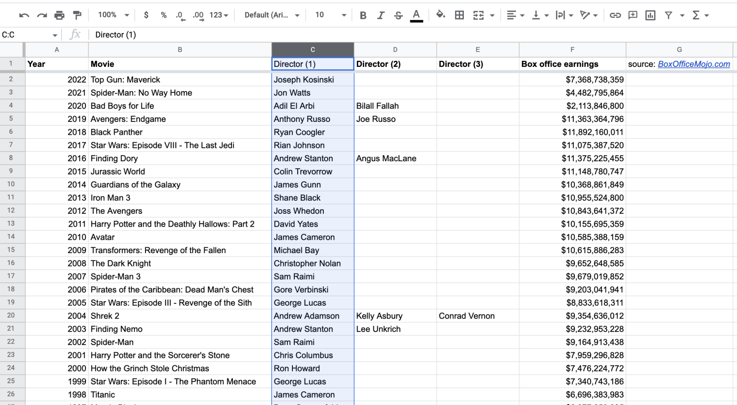
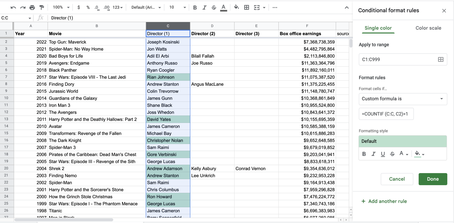
1. Highlight the column you want to find duplicates in.

Using our practice sheet, see if the Director (1) column has any duplicates.

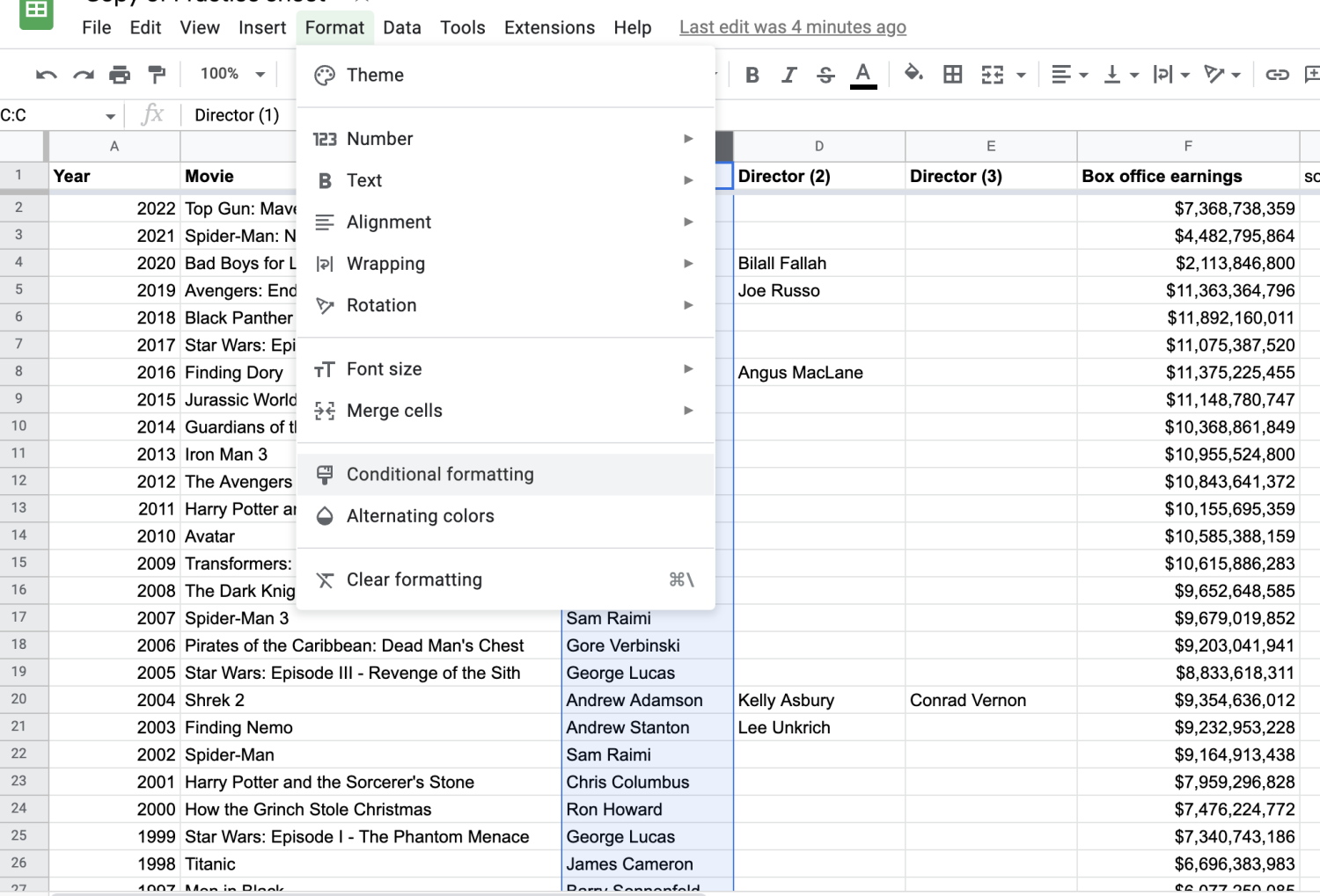
2. Click 'Format' in the top menu.

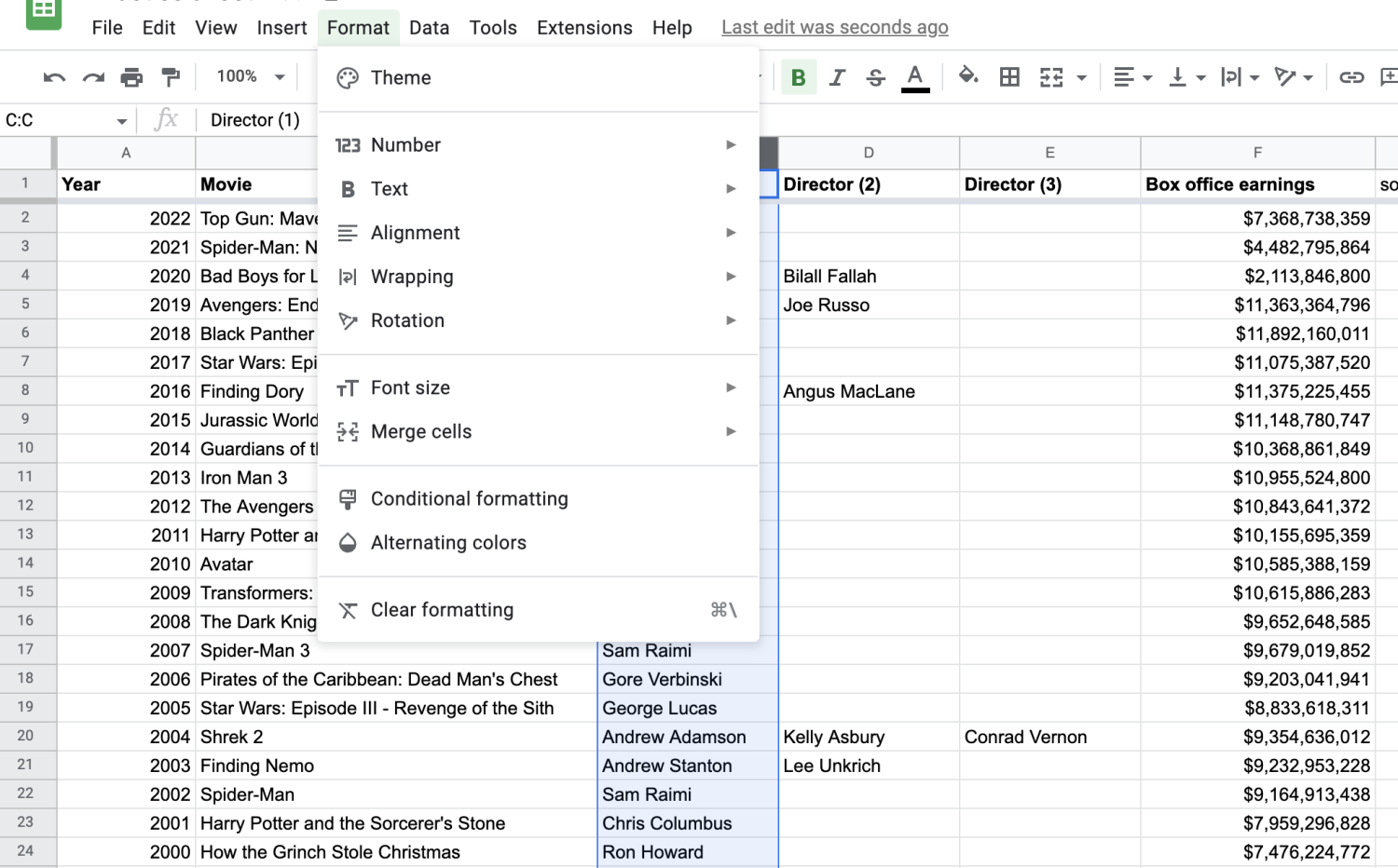
3. Click 'Conditional formatting.'

This will populate a box on the right-hand side of the screen. You’ll see a prompt called “Format cells if…” Click on that and scroll to the bottom.

4. In the 'Format cells if' box, click 'Custom formula is.'

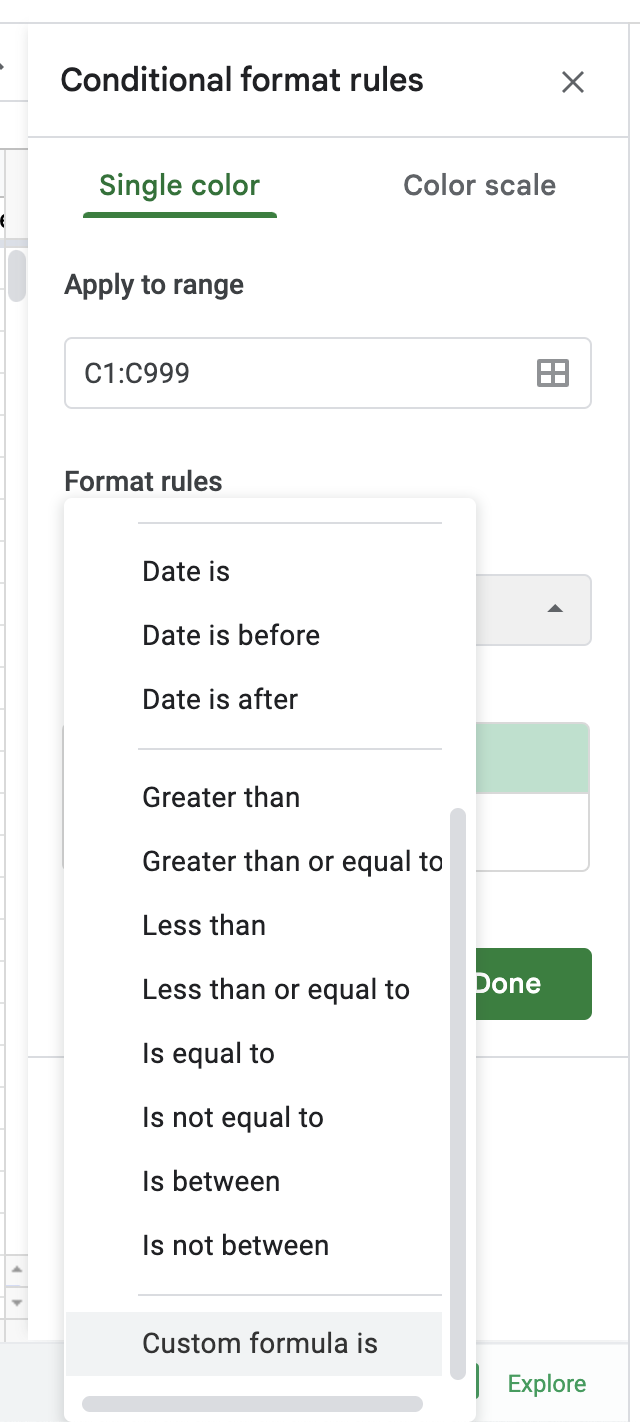
5. Use the COUNTIF formula to find duplicates.

The COUNTIF formula [=COUNTIF (A:A, A1)>1] tells Sheets where to look for duplicates. The information in the parentheses represents the column you want to track and the specific cell you want to start with. The information outside the parentheses states that you want Sheets to count duplicates or anything appearing more than once (>1). 

Since you're looking for duplicate directors, you want to adjust the formula to read the C column. Your formula should become =COUNTIF (C:C, C2)>1. You can see how it begins to highlight repeat directors.

How to find duplicates in Google Sheets with a browser add-on

TIP: If you’d rather not dive into formulas just yet, you can download an add-on from Google Sheets that will find and highlight duplicates for you.

How to highlight duplicate values in Google Sheets in multiple columns

Now that you know how to count duplicates in one column, learn how to adjust the process to count duplicates in multiple columns next.

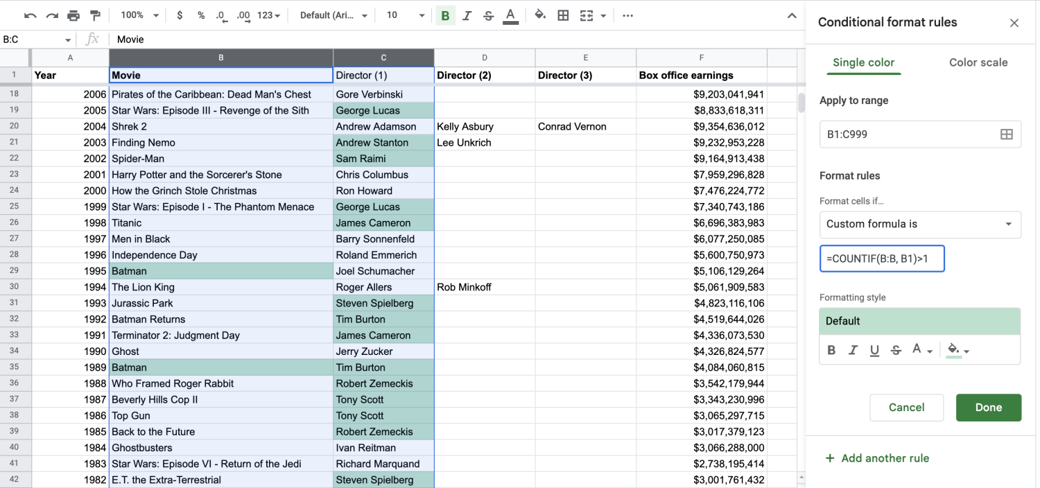
Let’s say you want to check movie titles and directors, so columns B and C in this case. We’ve purposely added an error in the titles column, repeating Batman twice. Clear any previous conditional format rules, and repeat the steps above until you get to the box where you’ll input your custom formula. 

You can go about this in two ways: 

1. Use 'Apply to range.'

By highlighting the columns you want to check, you’ll automatically tell Apply to range what to concentrate on, but you’ll have to adjust your custom formula to start with the value of that first column and first row. 

For your purposes, you’re looking at columns B and C, so your function should be =COUNTIF(B:B, B1)>1. That tells Sheets to start with B1 and go from there. 

You can adjust the range in Apply to range as needed. Let’s say you were looking at columns B and C, but now you want to include columns B through F. Rather than clear the conditional formatting, highlight your new columns, and start over, you can simply update the “Apply to range” to read “B1:F999.” 

Make sure the syntax of your formula matches the first value. For example, if you want to look at columns C through F now, you’ll update “Apply to range” to “C1:F999” and then make sure the function reads =COUNTIF(C:C, C1)>1. 

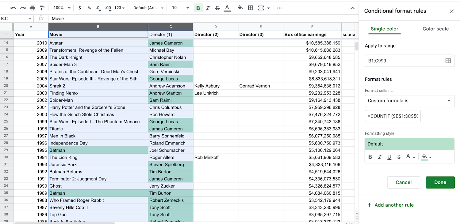
2. Use absolute values. 

Absolute values are a way to specify where Sheets should look for duplicates with the “$” symbol. You’ll need to frame every cell with a “$.” Our function becomes =COUNTIF ($B$1:$C$50, B1)>1. 

Learn more: Google Sheets vs. Excel: What's the Difference? 

How to highlight multiple columns using different colors

Performing these steps will highlight your duplicates using one color. But if you have multiple duplicates, you won't be able to see how many of each duplicate you have. 

In that case, you’d want to do a pivot table, which can help you see and better understand the relationship between data.

Build your data skills on Coursera

Whether you want to develop a new skill, get comfortable with an in-demand technology, or advance your abilities, keep growing with a Coursera Plus subscription. You’ll get access to over 10,000 flexible courses from over 350 top universities and companies.

订阅 Coursera Plus，培养就业技能

开始为期 7 天的免费试用

• 
• 
• 
• 

开始为期 7 天的免费试用